A Brief Introduction to Differential Privacy

A Brief Introduction to Differential Privacy

This article first appeared on the Georgian Impact Blog on Medium. https://medium.com/georgian-impact-blog/a-brief-introduction-to-differential-privacy-eacf8722283b

Aaruran Elamurugaiyan

Privacy can be quantified. Better yet, we can rank privacy-preserving strategies and say which one is more effective. Better still, we can design strategies that are robust even against hackers that have auxiliary information. And as if that wasn’t good enough, we can do all of these things simultaneously. These solutions, and more, reside in a probabilistic theory called differential privacy.

The Basics

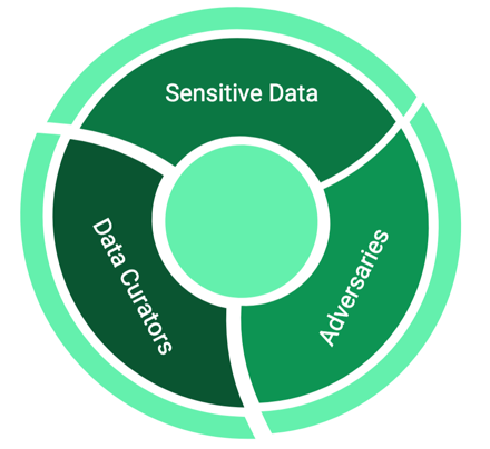
Here’s the context. We’re curating (or managing) a sensitive database and would like to release some statistics from this data to the public. However, we have to ensure that it’s impossible for an adversary to reverse-engineer the sensitive data from what we’ve released [1]. An adversary in this case is a party with the intent to reveal, or to learn, at least some of our sensitive data. Differential privacy can solve problems that arise when these three ingredients — sensitive data, curators who need to release statistics, and adversaries who want to recover the sensitive data — are present (see Figure 1). This reverse-engineering is a type of privacy breach.

But how hard is it to breach privacy? Wouldn’t anonymizing the data be good enough? If you have auxiliary information from other data sources, anonymization is not enough. For example, in 2007, Netflix released a dataset of their user ratings as part of a competition to see if anyone can outperform their collaborative filtering algorithm. The dataset did not contain personally identifying information, but researchers were still able to breach privacy; they recovered 99% of all the personal information that was removed from the dataset [2]. In this case, the researchers breached privacy using auxiliary information from IMDB.

How can anyone defend against an adversary who has unknown, and possibly unlimited, help from the outside world? Differential privacy offers a solution. Differentially-private algorithms are resilient to adaptive attacks that use auxiliary information [1]. These algorithms rely on incorporating random noise into the mix so that everything an adversary receives becomes noisy and imprecise, and so it is much more difficult to breach privacy (if it is feasible at all).

Noisy Counting

Let’s look at a simple example of injecting noise. Suppose we manage a database of credit ratings (summarized by Table 1).

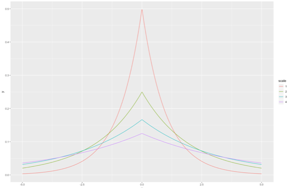
For this example, let’s assume that the adversary wants to know the number of people who have a bad credit rating (which is 3). The data is sensitive, so we cannot reveal the ground truth. Instead we will use an algorithm that returns the ground truth, N = 3, plus some random noise. This basic idea (adding random noise to the ground truth) is key to differential privacy. Let’s say we choose a random number L from a zero-centered Laplace distribution with standard deviation of 2. We return N+L. We’ll explain the choice of standard deviation in a few paragraphs. (If you haven’t heard of the Laplace distribution, see Figure 2). We will call this algorithm “noisy counting”.

If we’re going to report a nonsensical, noisy answer, what is the point of this algorithm? The answer is that it allows us to strike a balance between utility and privacy. We want the general public to gain some utility from our database, without exposing any sensitive data to a possible adversary.

What would the adversary actually receive? The responses are reported in Table 2.

The first answer the adversary receives is close to, but not equal to, the ground truth. In that sense, the adversary is fooled, utility is provided, and privacy is protected. But after multiple attempts, they will be able to estimate the ground truth. This “estimation from repeated queries” is one of the fundamental limitations of differential privacy [1]. If the adversary can make enough queries to a differentially-private database, they can still estimate the sensitive data. In other words, with more and more queries, privacy is breached. Table 2 empirically demonstrates this privacy breach. However, as you can see, the 90% confidence interval from these 5 queries is quite wide; the estimate is not very accurate yet.

How accurate can that estimate be? Take a look at Figure 3 where we’ve run a simulation several times and plotted the results [4].

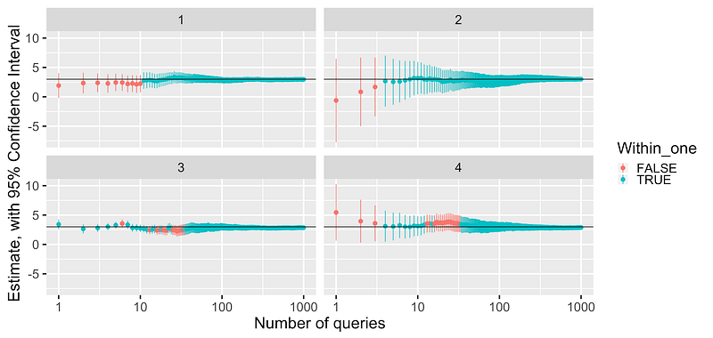
Each vertical line illustrates the width of a 95% confidence interval, and the points indicate the mean of the adversary’s sampled data. Note that these plots have a logarithmic horizontal axis, and that the noise is drawn from independent and identically distributed Laplace random variables. Overall, the mean is noisier with fewer queries (since the sample sizes are small). As expected, the confidence intervals become narrower as the adversary makes more queries (since the sample size increases, and the noise averages to zero). Just from inspecting the graph, we can see that it takes about 50 queries to make a decent estimate.

Let’s reflect on that example. First and foremost, by adding random noise, we made it harder for an adversary to breach privacy. Secondly, the concealing strategy we employed was simple to implement and understand. Unfortunately, with more and more queries, the adversary was able to approximate the true count.

If we increase the variance of the added noise, we can better defend our data, but we can’t simply add any Laplace noise to a function we want to conceal. The reason is that the amount of noise we must add depends on the function’s sensitivity, and each function has its own sensitivity. In particular, the counting function has a sensitivity of 1. Let’s take a look at what sensitivity means in this context.

Sensitivity and The Laplace Mechanism

For a function:

the sensitivity of f is:

on datasets D₁, D₂differing on at most one element [1].

The above definition is quite mathematical, but it’s not as bad as it looks. Roughly speaking, the sensitivity of a function is the largest possible difference that one row can have on the result of that function, for any dataset. For instance, in our toy dataset, counting the number of rows has a sensitivity of 1, because adding or removing a single row from any dataset will change the count by at most 1.

As another example, suppose we think about “count rounded up to a multiple of 5”. This function has a sensitivity of 5, and we can show this quite easily. If we have two datasets of size 10 and 11, they differ in one row, but the “counts rounded up to a multiple of 5” are 10 and 15 respectively. In fact, five is the largest possible difference this example function can produce. Therefore, its sensitivity is 5.

Calculating the sensitivity for an arbitrary function is difficult. A considerable amount of research effort is spent on estimating sensitivities [5], improving on estimates of sensitivity [6], and circumventing the calculation of sensitivity [7].

How does sensitivity relate to noisy counting? Our noisy counting strategy used an algorithm called the Laplace mechanism, which in turn relies on the sensitivity of the function it obscures [1] . In Algorithm 1, we have a naïve pseudocode implementation of the Laplace mechanism [1].

Algorithm 1

Input: Function F, Input X, Privacy level ϵ
Output: A Noisy Answer
Compute F (X)
Compute sensitivity of of F : S
Draw noise L from a Laplace distribution with variance:

Return F(X) + L

The larger the sensitivity S, the noisier the answer will be. Counting only has a sensitivity of 1, so we don’t need to add a lot of noise to preserve privacy.

Notice that the Laplace mechanism in Algorithm 1 consumes a parameter epsilon. We will refer to this quantity as the privacy loss of the mechanism and is part of the most central definition in the field of differential privacy: epsilon-differential privacy. To illustrate, if we recall our earlier example and use some algebra, we can see our noisy counting mechanism has epsilon-differential privacy, with an epsilon of 0.707. By tuning epsilon, we control the noisiness of our noisy counting. Choosing a smaller epsilon produces noisier results and better privacy guarantees. As a reference, Apple uses an epsilon of 2 in their keyboard’s differentially-private auto-correct [8].

The quantity epsilon is how differential privacy can provide rigorous comparisons between different strategies. The formal definition of epsilon-differential privacy is a bit more mathematically involved, so I have intentionally omitted it from this blog post. You can read more about it in Dwork’s survey of differential privacy [1].

As you recall, the noisy counting example had an epsilon of 0.707, which is quite small. But we still breached privacy after 50 queries. Why? Because with increased queries, the privacy budget grows, and therefore the privacy guarantee is worse.

The Privacy Budget

In general, the privacy losses accumulate[9]. When two answers are returned to an adversary, the total privacy loss is twice as large, and the privacy guarantee is half as strong. This cumulative property is a consequence of the composition theorem[9][10]. In essence, with each new query, additional information about the sensitive data is released. Hence, the composition theorem has a pessimistic view and assumes the worst-case scenario: the same amount of leakage happens with each new response. For strong privacy guarantees, we want the privacy loss to be small. So in our example where we have privacy loss of thirty-five(after 50 queries to our Laplace noisy-counting mechanism), the corresponding privacy guarantee is fragile.

How does differential privacy work if the privacy loss grows so quickly? To ensure a meaningful privacy guarantee, data curators can enforce a maximum privacy loss. If the number of queries exceeds the threshold, then the privacy guarantee becomes too weak and the curator stops answering queries. The maximum privacy loss is called the privacy budget [11]. We can think of each query as a privacy ‘expense’ which incurs an incremental privacy loss. The strategy of using budgets, expenses and losses is fittingly known as privacy accounting [11].

Privacy accounting is an effective strategy to compute the privacy loss after multiple queries, but it can still incorporate the composition theorem. As noted earlier, the composition theorem assumes the worst-case scenario. In other words, better alternatives exist.

Deep Learning

Deep learning is a sub-field of machine learning, that pertains to the training of deep neural networks (DNNs) to estimate unknown functions [11]. (At a high-level, a DNN is a sequence of affine and nonlinear transformations mapping some n-dimensional space to an m-dimensional space.) Its applications are widespread, and do not need to be repeated here. We will explore how to train a deep neural network privately.

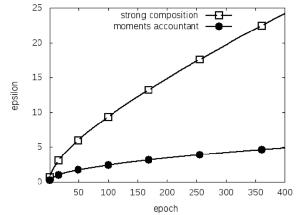
Deep neural networks are typically trained using a variant of stochastic gradient descent (SGD). Abadi et al. invented a privacy-preserving version of this popular algorithm, commonly referred to “private SGD” (or PSGD). Figure 4 illustrates the power in their novel technique [10]. Abadi et al. invented a new approach: the moments accountant. The basic idea behind the moments accountant is to accumulate the privacy expenditure by framing the privacy loss as a random variable, and using its moment-generating functions to better understand that variable’s distribution (hence the name) [10] . The full technical details are outside the scope of an introductory blog post, but we encourage you to read the original paper to learn more.

Final Thoughts

We’ve reviewed the theory of differential privacy and seen how it can be used to quantify privacy. The examples in this post show how the fundamental ideas can be applied and the connection between application and theory. It’s important to remember that privacy guarantees deteriorate with repeated use, so it’s worth thinking about how to mitigate this, whether that be with privacy budgeting or other strategies. You can investigate the deterioration by clicking this sentence and repeating our experiments. There are still many questions not answered here and a wealth of literature to explore — see the references below. We encourage you to read further.

References

[1] Cynthia Dwork. Differential privacy: A survey of results. International Conference on Theory and Applications of Models of Computation, 2008.

[2] Wikipedia Contributors. Laplace distribution, July 2018.

[3] Aaruran Elamurugaiyan. Plots demonstrating standard error of differentially private responses over number of queries., August 2018.

[4] Benjamin I. P. Rubinstein and Francesco Alda. Pain-free random differential privacy with sensitivity sampling. In 34th International Conference on Machine Learning (ICML’2017) , 2017.

[5] Adam Smith Kobi Nissim, Sofya Raskhodnikova. Smooth sensitivity and sampling in private data analysis. http://people.csail.mit.edu/asmith/PS/stoc321-nissim.pdf , June 2007. (Accessed on 08/03/2018).

[6] Kentaro Minami, HItomi Arai, Issei Sato, and Hiroshi Nakagawa. Differential privacy without sensitivity. In D. D. Lee, M. Sugiyama, U. V. Luxburg, I. Guyon, and R. Garnett, editors, Advances in Neural Information Processing Systems 29, pages 956–964. Curran Associates, Inc., 2016.

[7] Learning with Privacy at Scale. https://machinelearning.apple.com/docs/learning-with-privacy-at-scale/appledifferentialprivacysystem.pdf , 2017.

[8] Cynthia Dwork and Aaron Roth. The algorithmic foundations of differential privacy . Now Publ., 2014.

[9] Martin Abadi, Andy Chu, Ian Goodfellow, H. Brendan Mcmahan, Ilya Mironov, Kunal Talwar, and Li Zhang. Deep learning with differential privacy. Proceedings of the 2016 ACM SIGSAC Conference on Computer and Communications Security — CCS16 , 2016.

[10] Frank D. McSherry. Privacy integrated queries: An extensible platform for privacy-preserving data analysis. In Proceedings of the 2009 ACM SIGMOD International Conference on Management of Data , SIGMOD ’09, pages 19–30, New York, NY, USA, 2009. ACM.

[11] Wikipedia Contributors. Deep Learning, August 2018.