

An Introduction to Transfer Learning
A simple and concise explanation with real examples.
This article first appeared on the Georgian Impact Blog on Medium.
In this post, we lay down the foundations of transfer learning. We start by explaining the underlying idea behind transfer learning and its formal definition. Then we will discuss transfer learning problems and existing solutions. Finally, we will briefly take a look at some transfer learning use-cases.
In the next posts in this series, we will use the notations and definitions described here and dive deeper into recent trends in the field and look at how transfer learning is being used to solve real-world problems. Follow the Georgian Impact Blog to make sure you don’t miss these posts.
Table of contents — click on the links to skip ahead:
- What is Transfer Learning?
- Mathematical Notations and Definitions
- Categorization of Transfer Learning Problems
- Categorization of Transfer Learning Solutions
- Real Applications of Transfer Learning
- Extra Resources for Diving Deep on Transfer Learning
What is Transfer Learning?
As humans, we find it easy to transfer knowledge we have learned from one domain or task to another. When we encounter a new task, we don’t have to start from scratch. Instead, we use our previous experience to learn and adapt to that new task faster and more accurately[1].
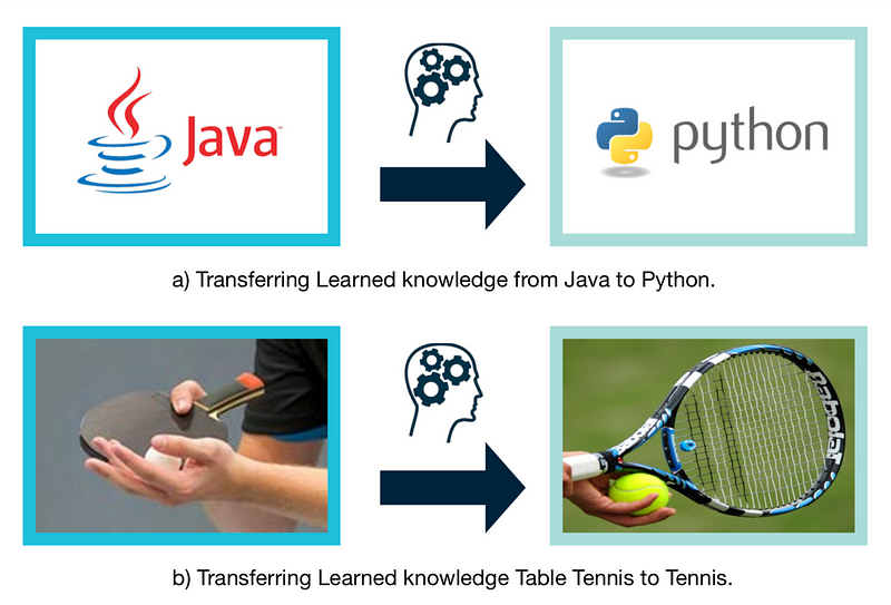
For example, if you have any experience programming with Java, C/C# or any other programming languages, you’re already familiar with concepts like loops, recursion, objects and etc (Figure 1, a). If you then try to pick up a new programming language like python, you don’t need to learn these concepts again, you just need to learn the corresponding syntax. Or to take another example, if you have played table tennis a lot it will help you learn tennis faster as the strategies in these games are similar (Figure 1, b).
In recent years, fuelled by the advances in supervised and unsupervised machine learning, we have seen astonishing leaps in the application of artificial intelligence. We have reached a stage that we can build autonomous vehicles, intelligent robots and cancer detection systems with human-level or even super-human performance (Figure 2).https://georgian.io/media/5ff23bbbefc2941da7d89bfb475b0758Figure 2. Advances in Artificial Intelligence in recent years.
Despite the remarkable results, these models are data hungry and their performance relies heavily on the quality and size of training data. However, in real-world scenarios, large amounts of labeled data are usually expensive to obtain or not available which means performance is low or projects are abandoned entirely. What’s more, these models still lack the ability to generalize to any situation beyond those they encountered during training[2], so they are limited in what they can achieve.
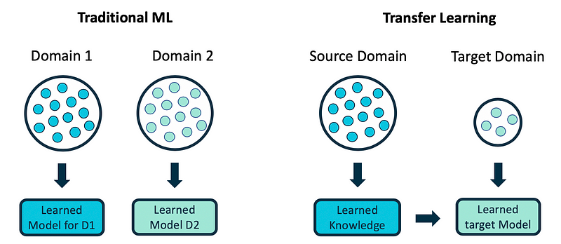
Inspired by the human capability to transfer knowledge, the machine learning community has turned their focus to transfer learning to overcome these issues. Unlike the traditional machine learning paradigm where the learning process happens in isolation, without considering knowledge from any other domain (Figure 3 left side), transfer learning uses knowledge from other existing domains (source) during the learning process for a new domain (target) (Figure 3 right side).
Transfer learning addresses these three questions:
- What information in the source is useful and transferable to target?
- What is the best way of transferring this information?
- How to avoid transferring information that is detrimental to the desired outcome?
The answer to these questions depends on the similarities between the feature spaces, models and tasks of the target and source domains[1]. We will provide examples below to describe these concepts.
Mathematical Notations and Definitions in Transfer Learning
In this section, we will briefly discuss the standard notations and definitions used for transfer learning in the research community[1, 3]. In the remainder of the post, we use these notations and definitions to dive deeper into more technical topics, so it’s worth going a little slower through this section.
Notation
Domain: A domain 𝔇 = {𝑋, P(X)} is defined by two components:
- A feature space 𝑋
- and a marginal probability distribution P(X)whereX={𝑥₁, 𝑥₂, 𝑥₃, …, 𝑥𝚗} ∈ 𝑋
If two domains are different, then they either have different feature spaces (𝑋t ≠ 𝑋s) or different marginal distributions (P(Xt) ≠ P(Xs)).
Task: Given a specific domain 𝔇, a task 𝒯={𝑌, 𝒇(.)} consists of two parts:
- A label space 𝑌
- and a predictive function 𝒇(.), which is not observed but can be learned from training data {(𝑥ᵢ, 𝑦ᵢ)| i ∈ {1, 2, 3, …, N}, where 𝑥ᵢ ∈ 𝑋 and 𝑦ᵢ ∈ 𝑌 }. From a probabilistic viewpoint 𝒇(𝑥ᵢ), can also be written as p(𝑦ᵢ|𝑥ᵢ), so we can rewrite task 𝒯as 𝒯={𝑌, P(𝖸|X)}.
In general, if two tasks are different, then they may have different label spaces(𝑌t ≠ 𝑌s) or different conditional probability distributions (P(𝖸t|Xt) ≠ P(𝖸s|Xs)).
Definition
Given a source domain 𝔇s and corresponding learning task 𝒯s, a target domain 𝔇t and learning task 𝒯t, transfer learning aims to improve the learning of the conditional probability distribution P(𝖸t|Xt) in 𝔇t with the information gained from 𝔇s and 𝒯s, where 𝔇t ≠ 𝔇s or 𝒯t ≠ 𝒯s. For simplicity, we only used a single source domain in the definition above, but the idea can be extended to multiple source domains.
If we take this definition of domain and task, then we will have either 𝔇t ≠ 𝔇s or 𝒯t ≠ 𝒯s, which results in four common transfer learning scenarios[3]. We will explain these scenarios below in the context of two popular machine learning tasks, part of speech (POS) tagging, and object classification.
POS tagging is the process of associating a word in a corpus with its corresponding part of speech tag, based on its context and definition. For example: In the sentence “My name is Azin.” ‘My’ is a ‘PRP’, ‘name’ is ‘NN’, ‘is’ is ‘VBZ’, and ‘Azin’ is ‘NNP’. Object classification is the process of classifying the objects seen in an image to the set of defined classes like apple, bus, forest etc. Let’s take a look at the following four cases with these tasks in mind.
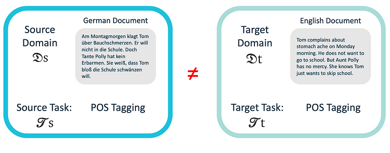
- 𝑋t ≠ 𝑋s
Let’s say that we would like to do POS tagging in German documents (𝒯t). Assuming that the basics of Germany and English are similar in grammar and structure, we can leverage the knowledge learned from thousands of existing rich English datasets (𝔇s) for this task (Figure 4), even though our features spaces (English and German words) are completely different (𝑋t ≠ 𝑋s). Another example is using tags and descriptions (𝔇s) provided alongside images to improve the object classification task (𝒯t) where text and images are presented in completely different features spaces (𝑋t ≠ 𝑋s). - P(Xt) ≠ P(Xs)
Let’s say that we would like to do POS tagging in English documents (𝒯t) and we would like to use readily available English datasets for this. Although these documents are written in the same language (𝑋t = 𝑋s), they focus on different topics, and so the frequency of the words used (features) is different. For example, in a cooking document, “tasty” or “delicious” might be common, but they would be rarely used in a technical document. Words that are generic and domain-independent occur at a similar rate in both domains. However, words that are domain-specific are used more frequently in one domain because of the strong relationship with that domain topic. This is referred to as frequency feature bias and will cause the marginal distributions between the source and target domains to be different. Another example is using cartoon images to improve object classification for photo images. They are both images so the features spaces are the same (𝑋t =𝑋s), however, the colors and shapes in cartoons are very different to photos (P(Xt) ≠ P(Xs)). This scenario is generally referred to as domain adaptation. - 𝑌t ≠ 𝑌sLet’s say we want to do POS tagging with a customized set of tags (𝒯t) which is different from tags in other existing datasets. In this case, the target and source domains have different label spaces (𝑌t ≠ 𝑌s). Another example would be using a data set with different object classes (cat and dog) to improve object classification for a specific set of classes (chair, desk, and human).
- P(𝖸t|Xt) ≠ P(𝖸s|Xs)
In POS tagging the source and target can have the same language(𝑋t = 𝑋s), the same number of classes (𝑌t =𝑌s), and same frequency of words
(P(Xt)=P(Xs)), but individual words can have different meanings in the source and target (P(𝖸t|Xt) ≠ P(𝖸s|Xs)). A specific example is the word “monitor.” In one domain (technical reports) it might be used more frequently as a noun and in another domain (patient monitoring reports), it might be used predominantly as a verb. This is another form of bias which is referred to as context feature bias and it causes the conditional distributions to be different between the source and target. Similarly, in an image, if a piece of bread is hung on a refrigerator it is most likely to be a magnet, however, if it is close to a pot of jam it is more likely to be a piece of bread.
One final case that does not sit well in any of the four above (based on our definitions) but that can cause a difference between the source and target is P(𝖸t) ≠ P(𝖸s). For example, the source dataset may have completely balanced binary samples, but the target domain may have 90% positive and only 10% negative samples. There are different techniques for addressing this issue, such as down-sampling and up-sampling, and SMOTE[4].
Categorization of Transfer Learning Problems
When you read the literature on transfer learning, you’ll notice that the terminology and definitions are often inconsistent. For example, domain adaptation and transfer learning are sometimes used to refer to the same concept. Another common inconsistency is how transfer learning problems are grouped together. Traditionally transfer learning problems were categorized into three main groups based on the similarity between domains and also the availability of labeled and unlabeled data[1]: Inductive transfer learning, transductive transfer learning, and unsupervised transfer learning.
However, thanks to developments in deep learning, the recent body of research in this field, has broadened the scope of transfer learning and a new and more flexible taxonomy[3] has emerged. This taxonomy generally categorizes transfer learning problems into two main classes based on the similarity of domains, regardless of the availability of labeled and unlabeled data[3]: Homogeneous transfer learning and heterogeneous transfer learning. We will explore this taxonomy below.
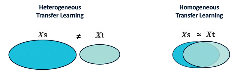
1. Homogeneous Transfer Learning
In homogeneous transfer learning (Figure 5 right side), we have the situation where 𝑋t = 𝑋s and 𝑌t = 𝑌s. Therefore, we want to bridge the gap in the data distributions between the source and target domains, i.e. address P(Xt) ≠ P(Xs)and/or P(𝖸t|Xt) ≠ P(𝖸s|Xs). The solutions to homogeneous transfer learning problems use one of the following general strategies:
- Trying to correct for the marginal distribution differences in the source and target ( P(Xt) ≠ P(Xs)).
- Trying to correct for the conditional distribution difference in the source and target (P(𝖸t|Xt) ≠ P(𝖸s|Xs)).
- Trying to correct both the marginal and conditional distribution differences in the source and target.
2. Heterogeneous Transfer Learning
In heterogeneous transfer learning, the source and target have different feature spaces 𝑋t ≠ 𝑋s (generally non-overlapping) and/or 𝑌t ≠ 𝑌s, as the source and target domains may share no features and/or labels (Figure 5 left side). Heterogeneous transfer learning solutions bridge the gap between feature spaces and reduce the problem to a homogeneous transfer learning problem where further distribution (marginal or conditional) differences will need to be corrected.
Another important concept to discuss is negative transfer. If the source domain is not very similar to the target domain, the information learned from the source can have a detrimental effect on a target learner. This is referred to as negative transfer.
In the rest of the post, we will describe the existing methods for homogeneous and heterogeneous transfer learning. We’ll also discuss some techniques to avoid negative transfer.
Categorization of Transfer Learning Solutions
Solutions for the two main categories of transfer learning problems above can be summarized into five different classes based on what is being transferred:
Homogeneous Transfer Learning
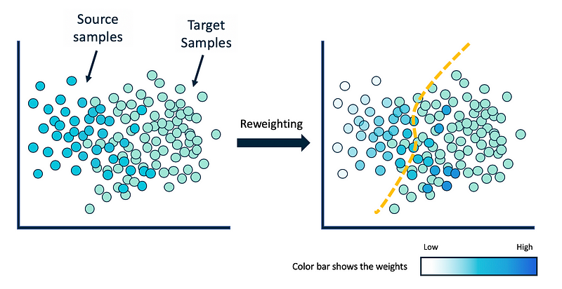
1.Instance-based Approaches: Instance-based transfer learning methods try to reweight the samples in the source domain in an attempt to correct for marginal distribution differences[4, 5, 6]. These reweighted instances are then directly used in the target domain for training. Using the reweighted source samples helps the target learner to use only the relevant information from the source domain. These methods work best when the conditional distribution is the same in both domains.
Instance-based approaches differ in their weighting strategies. For example, the method in Correcting Sample Selection Bias by Unlabeled Data (Huang et al.) [7] finds and applies the weight that matches up the mean of the target and source domains. Another common solution is to train a binary classifier that separates source samples from target samples and then use this classifier to estimate the source sample weights (Figure 6). This method gives a higher weight to the source samples that are more similar to target samples.
2. Feature-based Approaches: Feature-based approaches are applicable to both homogeneous and heterogeneous problems. With heterogeneous problems, the main goal of using these methods is to reduce the gap between feature spaces of source and target[10, 11, 14, 15]. With homogeneous problems, these methods aim to reduce the gap between the marginal and conditional distributions of the source and target domains[8, 9, 12, 13]. Feature-based transfer learning approaches fall into two groups:
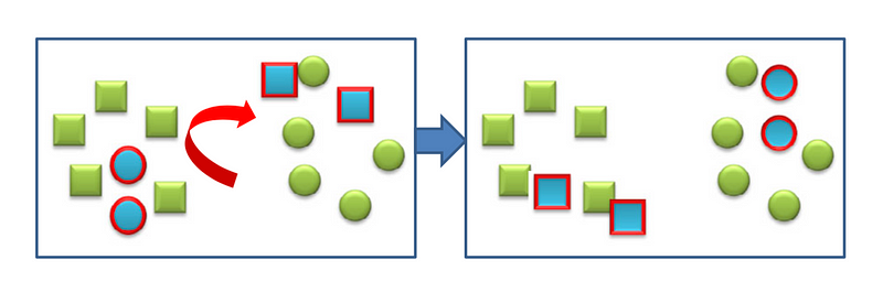
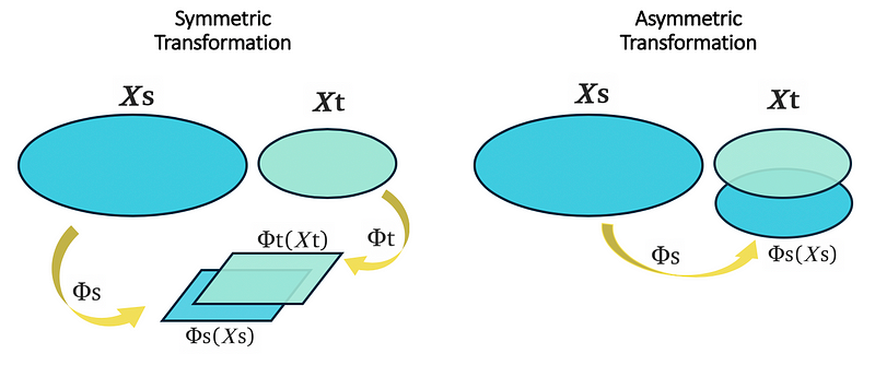
- Asymmetric Feature Transformation: This approach employs a transformation (Φs/Φt) to transform one of the domains (source/target) to the other one (target/source)[8, 9, 25]. This method works the best when the source and target domains have the same label spaces and one can transform them without context feature bias (Figure 8 right side). Figure 7, shows the asymmetric feature-based method as presented in Asymmetric and Category Invariant Feature Transformations for Domain Adaptation (Hoffman et al.) [25]. This method tries to transform the source domain (blue samples) so that the distance between similar samples in source and target domains is minimized.
- Symmetric Feature Transformation: This approach discovers underlying meaningful structures by transforming both of the domains to a common latent feature space — usually of a low dimension — that has predictive qualities while reducing the marginal distribution between the domains (Figure 8 left side)[12, 13]. Although the high-level goal behind these methods (improving the performance of a target learner) is very different from the objective in representation learning, the idea behind them is fairly close[23].
3. Parameter-based Approaches:
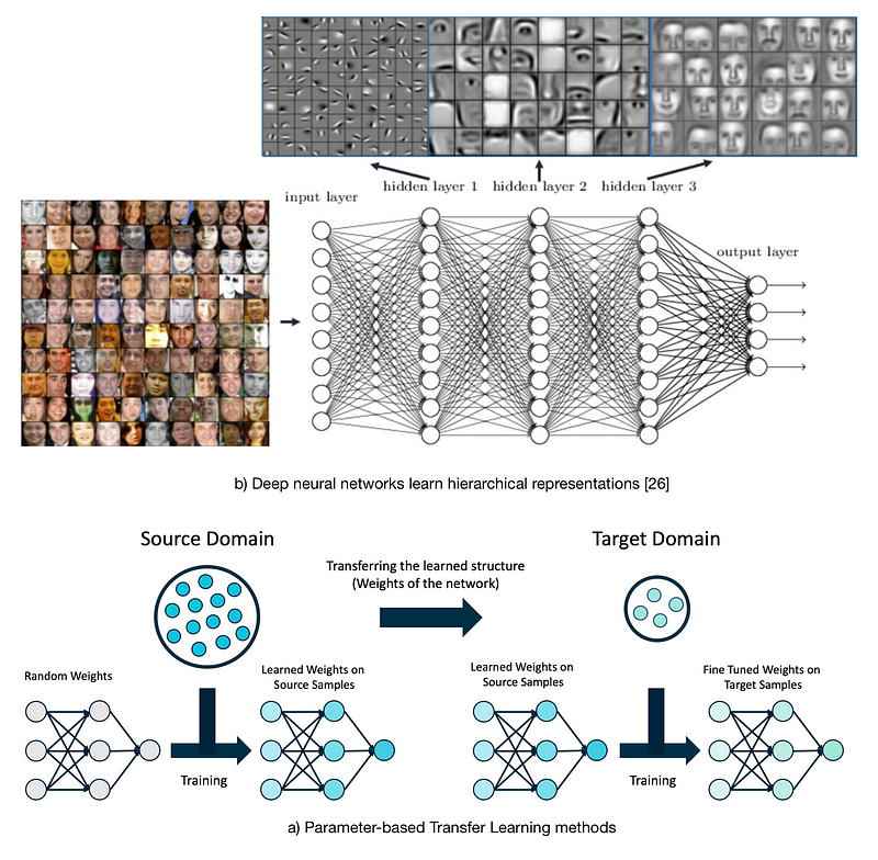
This category of transfer learning tries to transfer knowledge through the shared parameters of the source and target domain learner models[16, 17]. Some of these methods also transfer the learned knowledge by creating multiple source learner models and optimally combining the reweighted learners (ensemble learners) to form an improved target learner. The idea behind parameter-based methods is that a well-trained model on the source domain has learned a well-defined structure, and if two tasks are related, this structure can be transferred to the target model.
The concept of sharing parameters (weights) has been widely used in deep learning models. In general, there are two ways to share the weights in deep learning models, soft weight sharing, and hard weight sharing. In soft weight sharing, the model is usually penalized if its weights deviate significantly from a given set of weights[18]. In hard weight sharing, the exact weights are shared among different models[19]. Very commonly hard weight sharing uses previously trained weights as the starting weights of a deep learning model.
Usually, when training a deep neural network, the model starts with randomly initialized weights close to zero and adapts its weights as it sees more and more training samples. However, training a deep model in this way requires a lot of time and effort to collect and label data. That’s why it’s so advantageous to start with the previously trained weights from another similar domain (source) and then fine-tune the weights specifically for a new domain (target). This can potentially save time and reduce the costs since fine-tuning requires much less labeled data. It’s also been shown that this approach can help with robustness. Figure 9, demonstrates this method.
4. Hybrid-based Approaches (Instance and Parameter): This category focuses on transferring knowledge through both instances and shared parameters. This is a relatively new approach and a lot of interesting research is emerging [20].
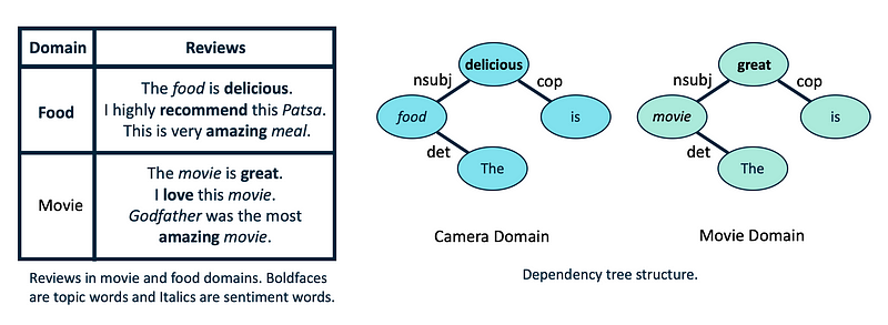
5. Relational-based Approaches: The last transfer learning category (and also the newest) is to transfer the knowledge through learning the common relationships between the source and target domains[21, 22]. In the following, we provide an example here in the context of sentiment analysis.
As you see in Figure 10,the frequency of used words in different review domains (here Movie and Food) is very different, but the structure of the sentences is fairly similar. Therefore, if we learn the relationship between different parts of the sentence in the Food domain, it can help significantly with analyzing the sentiment in another domain (here Movie)[21].
Heterogeneous Transfer Learning
Since in heterogeneous transfer learning problems the features spaces are not equivalent, the only class of transfer learning solutions that can be applied to this category is the feature-based methods[10, 11, 14, 15]described above (Figure 8). After reducing the gap between features spaces by using symmetric[10, 11] or asymmetric[14, 15] feature-based methods and converting a heterogeneous problem to a homogeneous problem, the other four classes of transfer learning solutions can be applied to further correct the distribution differences between target and source domains.
Summary
Figure 11 shows the different categories of transfer learning problems and solutions. As you can see, some classes of transfer learning solutions (instance-based, feature-based, and relational-based methods) transfer the knowledge at the data level while some classes (parameter-based methods) transfer the knowledge at the model level.

Real Applications of Transfer Learning
One of the biggest challenges that SaaS/AI companies often face when onboarding a new customer is the lack of labeled data to build a machine learning model for the new customer, which is referred to as cold-start. Even after collecting data, which can potentially take several months to years, there are other issues like sparsity and imbalance problems that make it hard to build a model with acceptable performance. When a model uses sparse and imbalanced data, it is often not sufficiently expressive and performs poorly especially on minority classes.
The aforementioned issues negatively affect customers acquisition and retention and make it extremely difficult for SaaS/AI companies to scale efficiently. Transfer learning can overcome these issues by leveraging existing information from other customers (source domain) when building the model for the new customer (target domain), Figure 12.
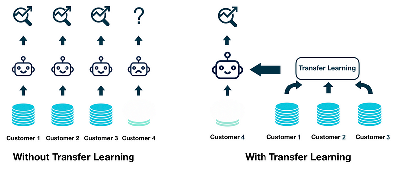
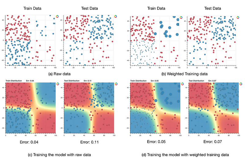
Figure 13 illustrates another machine learning challenge that can be addressed by transfer learning — domain shift[24]. Supervised machine learning models still lack the ability to generalize to conditions that are different from the ones encountered during training. In other words, when the statistical characteristics of the training data and the test data are different (domain shift) (Figure 13-(a)), we often experience performance deterioration or collapse as the model doesn’t know how to generalize to the new situation (Figure 13-(c)). Transfer learning (domain adaptation)methods can help to address this issue by reducing the gap between the two domains and consequently improving the performance of the model on the test data (Figure 13-(d)).
There are many other applications of transfer learning in the real world. Problems like learning from simulation in robotics and autonomous driving, transferring knowledge across different languages and so on are all examples. In our next post, we will discuss recent studies and developments in transfer learning and their application to real-world problems in greater detail.
If you have any questions or remarks, we’d love to hear from you! Please feel free to contact us — leave a comment below or reach out to us on Twitter.
Extra Resources for Diving Deep on Transfer Learning
[1] Pan, S. J., & Yang, Q. (2010). A Survey on Transfer Learning. IEEE Transactions on Knowledge and Data Engineering, 22(10), 1345–1359. doi:10.1109/tkde.2009.191
[2] Ruder, S. (2018, October 24). Transfer Learning — Machine Learning’s Next Frontier. Retrieved from http://ruder.io/transfer-learning/
[3] Weiss, K., Khoshgoftaar, T. M., & Wang, D. (2016). A survey of transfer learning. Journal of Big Data, 3(1). doi:10.1186/s40537–016–0043–6
[4] Chawla, N. V., Bowyer, K. W., Hall, L. O., & Kegelmeyer, W. P. (2002). SMOTE: Synthetic Minority Over-sampling Technique. Journal of Artificial Intelligence Research, 16, 321–357. doi:10.1613/jair.953
[5] Yao, Y., & Doretto, G. (2010). Boosting for transfer learning with multiple sources. 2010 IEEE Computer Society Conference on Computer Vision and Pattern Recognition. doi:10.1109/cvpr.2010.5539857
[6] Asgarian, A., Sobhani, P., Zhang, J. C., Mihailescu, M., Sibilia, A., Ashraf, A. B., Taati, B. (2018). Hybrid Instance-based Transfer Learning Method.
Machine Learning for Health (ML4H) Workshop at Neural Information Processing Systems arXiv:cs/0101200
[7] Huang, J., Gretton, A., Borgwardt, K., Schölkopf, B., & Smola, A. J. (2007). Correcting sample selection bias by unlabeled data. In Advances in neural information processing systems(pp. 601–608).
[8] Long, M., Wang, J., Ding, G., Pan, S. J., & Philip, S. Y. (2014). Adaptation regularization: A general framework for transfer learning. IEEE Transactions on Knowledge and Data Engineering, 26(5), 1076–1089.
[9] Long, M., Wang, J., Ding, G., Sun, J., & Yu, P. S. (2013). Transfer feature learning with joint distribution adaptation. In Proceedings of the IEEE international conference on computer vision (pp. 2200–2207).
[10] Sukhija, S., Krishnan, N. C., & Singh, G. (2016, July). Supervised Heterogeneous Domain Adaptation via Random Forests. In IJCAI (pp. 2039–2045).
[11] Feuz, K. D., & Cook, D. J. (2015). Transfer learning across feature-rich heterogeneous feature spaces via feature-space remapping (FSR). ACM Transactions on Intelligent Systems and Technology (TIST), 6(1), 3.
[12] Oquab, M., Bottou, L., Laptev, I., & Sivic, J. (2014). Learning and transferring mid-level image representations using convolutional neural networks. In Proceedings of the IEEE conference on computer vision and pattern recognition (pp. 1717–1724).
[13] Pan, S. J., Tsang, I. W., Kwok, J. T., & Yang, Q. (2011). Domain adaptation via transfer component analysis. IEEE Transactions on Neural Networks, 22(2), 199–210.
[14] Samat, A., Persello, C., Gamba, P., Liu, S., Abuduwaili, J., & Li, E. (2017). Supervised and semi-supervised multi-view canonical correlation analysis ensemble for heterogeneous domain adaptation in remote sensing image classification. Remote sensing, 9(4), 337.
[15] Duan, L., Xu, D., & Tsang, I. (2012). Learning with augmented features for heterogeneous domain adaptation. arXiv preprint arXiv:1206.4660.
[16] Duan, L., Xu, D., & Chang, S. F. (2012, June). Exploiting web images for event recognition in consumer videos: A multiple source domain adaptation approach. In 2012 IEEE Conference on Computer Vision and Pattern Recognition (pp. 1338–1345). IEEE.
[17] Yao, Y., & Doretto, G. (2010, June). Boosting for transfer learning with multiple sources. In 2010 IEEE Computer Society Conference on Computer Vision and Pattern Recognition (pp. 1855–1862). IEEE.
[18] Rozantsev, A., Salzmann, M., & Fua, P. (2018). Beyond sharing weights for deep domain adaptation. IEEE transactions on pattern analysis and machine intelligence.
[19] Meir, B. E., & Michaeli, T. (2017). Joint auto-encoders: a flexible multi-task learning framework. arXiv preprint arXiv:1705.10494.
[20] Xia, R., Zong, C., Hu, X., & Cambria, E. (2013). Feature ensemble plus sample selection: domain adaptation for sentiment classification. IEEE Intelligent Systems, 28(3), 10–18.
[21] Li, F., Pan, S. J., Jin, O., Yang, Q., & Zhu, X. (2012, July). Cross-domain co-extraction of sentiment and topic lexicons. In Proceedings of the 50th Annual Meeting of the Association for Computational Linguistics: Long Papers-Volume 1 (pp. 410–419). Association for Computational Linguistics.
[22] Yang, Z., Dhingra, B., He, K., Cohen, W. W., Salakhutdinov, R., & LeCun, Y. (2018). Glomo: Unsupervisedly learned relational graphs as transferable representations. arXiv preprint arXiv:1806.05662.
[23] Ganin, Y., & Lempitsky, V. (2014). Unsupervised domain adaptation by backpropagation. arXiv preprint arXiv:1409.7495.
[24] Quiñonero-Candela, J. (2009). Dataset shift in machine learning. Cambridge, MA: MIT Press.
[25] Hoffman, J., Rodner, E., Donahue, J., Kulis, B., & Saenko, K. (2014). Asymmetric and category invariant feature transformations for domain adaptation. International journal of computer vision, 109(1–2), 28–41.
[26] Exploring Deep Learning & CNNs. (2018, December 16). Retrieved from https://www.rsipvision.com/exploring-deep-learning/
Read more like this
Testing LLMs for trust and safety
We all get a few chuckles when autocorrect gets something wrong, but…
Introducing Georgian’s “Crawl, Walk, Run” Framework for Adopting Generative AI
Since its founding in 2008, Georgian has conducted diligence on hundreds of…